Introduction to hacksig • hacksig

Hacksig is a collection of cancer transcriptomics gene signatures and it provides a simple and tidy interface to compute single sample enrichment scores.

This document will show you how to getting started with hacksig, but first, we must load the following packages:

library(hacksig)

# to plot and transform data
library(dplyr)
library(ggplot2)
library(purrr)
library(tibble)
library(tidyr)

# to get the MSigDB gene signatures
library(msigdbr)

# to parallelize computations
library(future)

theme_set(theme_bw())

Available signatures from the literature

In order to get a complete list of the implemented signatures, you can use get_sig_info(). It returns a tibble with very useful information:

the signature_id;
a string of keywords associated to a signature (separated by the “pipe” | symbol);
the publication_doi linking to the original publication;
a brief description.

get_sig_info()
#> # A tibble: 40 × 4
#>   signature_id       signature_keywords                          publi…¹ descr…²
#>   <chr>              <chr>                                       <chr>   <chr>  
#> 1 ayers2017_immexp   ayers2017_immexp|immune expanded            10.117… Immune…
#> 2 bai2019_immune     bai2019_immune|head and neck squamous cell… 10.115… Immune…
#> 3 cinsarc            cinsarc|metastasis|sarcoma|sts              10.103… Biomar…
#> 4 dececco2014_int172 dececco2014_int172|head and neck squamous … 10.109… Signat…
#> 5 eschrich2009_rsi   eschrich2009_rsi|radioresistance|radiosens… 10.101… Genes …
#> # … with 35 more rows, and abbreviated variable names ¹publication_doi,
#> #   ²description

If you want to get the list of gene symbols for one or more of the implemented signatures, then use get_sig_genes() with valid keywords:

get_sig_genes("ifng")
#> $muro2016_ifng
#> [1] "CXCL10"  "CXCL9"   "HLA-DRA" "IDO1"    "IFNG"    "STAT1"

Check your signatures

The first thing you should do before computing scores for a signature is to check how many of its genes are present in your data. To accomplish this, we can use check_sig() on a normalized gene expression matrix (either microarray or RNA-seq normalized data), which must be formatted as an object of class matrix or data.frame with gene symbols as row names and sample IDs as column names.

For this tutorial, we will use test_expr (an R object included in hacksig) as an example gene expression matrix with 20 simulated samples.

By default, check_sig() will compute statistics for every signature implemented in hacksig.

check_sig(test_expr)
#> # A tibble: 40 × 5
#>   signature_id     n_genes n_present frac_present missing_genes
#>   <chr>              <int>     <int>        <dbl> <list>       
#> 1 wu2020_metabolic      30        20        0.667 <chr [10]>   
#> 2 muro2016_ifng          6         4        0.667 <chr [2]>    
#> 3 liu2020_immune         6         4        0.667 <chr [2]>    
#> 4 liu2021_mgs            6         4        0.667 <chr [2]>    
#> 5 lu2020_npc             3         2        0.667 <chr [1]>    
#> # … with 35 more rows

You can filter for specific signatures by entering keywords in the signatures argument (partial matching and regular expressions will work too):

check_sig(test_expr, signatures = c("metab", "cinsarc"))
#> # A tibble: 2 × 5
#>   signature_id     n_genes n_present frac_present missing_genes
#>   <chr>              <int>     <int>        <dbl> <list>       
#> 1 wu2020_metabolic      30        20        0.667 <chr [10]>   
#> 2 cinsarc               67        40        0.597 <chr [27]>

We can also check for signatures not implemented in hacksig, that is custom signatures. For example, we can use the msigdbr package to download the Hallmark gene set collection as a tibble and transform it into a list:

hallmark_list <- msigdbr(species = "Homo sapiens", category = "H") %>%
    distinct(gs_name, gene_symbol) %>%
    nest(genes = c(gene_symbol)) %>%
    mutate(genes = map(genes, compose(as_vector, unname))) %>%
    deframe()

check_sig(test_expr, hallmark_list)
#> # A tibble: 50 × 5
#>   signature_id                        n_genes n_present frac_present missing_g…¹
#>   <chr>                                 <int>     <int>        <dbl> <list>     
#> 1 HALLMARK_WNT_BETA_CATENIN_SIGNALING      42        27        0.643 <chr [15]> 
#> 2 HALLMARK_APICAL_SURFACE                  44        28        0.636 <chr [16]> 
#> 3 HALLMARK_BILE_ACID_METABOLISM           112        70        0.625 <chr [42]> 
#> 4 HALLMARK_NOTCH_SIGNALING                 32        20        0.625 <chr [12]> 
#> 5 HALLMARK_PI3K_AKT_MTOR_SIGNALING        105        65        0.619 <chr [40]> 
#> # … with 45 more rows, and abbreviated variable name ¹missing_genes

Missing genes for the HALLMARK_NOTCH_SIGNALING gene set are:

check_sig(test_expr, hallmark_list) %>% 
    filter(signature_id == "HALLMARK_NOTCH_SIGNALING") %>% 
    pull(missing_genes)
#> [[1]]
#>  [1] "FZD5"    "HEYL"    "KAT2A"   "MAML2"   "NOTCH1"  "NOTCH3"  "PPARD"  
#>  [8] "PRKCA"   "PSEN2"   "SAP30"   "ST3GAL6" "TCF7L2"

Compute single sample scores

hack_sig

The main function of the package, hack_sig(), permits to obtain single sample scores from gene signatures. By default, it will compute scores for all the signatures implemented in the package with the original publication method.

hack_sig(test_expr)
#> Warning: ℹ No genes are present in 'expr_data' for the following signatures:
#> ✖ zhu2021_ferroptosis
#> ✖ rooney2015_cyt
#> ℹ To obtain CINSARC, ESTIMATE and Immunophenoscore with the original procedures, see:
#> ?hack_cinsarc
#> ?hack_estimate
#> ?hack_immunophenoscore
#> # A tibble: 20 × 32
#>   sample_id ayers2017_…¹ bai20…² decec…³ eschr…⁴ eusta…⁵ fan20…⁶ fang2…⁷ han20…⁸
#>   <chr>            <dbl>   <dbl>   <dbl>   <dbl>   <dbl>   <dbl>   <dbl>   <dbl>
#> 1 sample1           5.71   -22.3    2.62  0.0289    8.1   -2.67     2.96  -0.503
#> 2 sample10          6.96   -23.0    2.69  0.415     8.17  -0.743    3.42  -0.259
#> 3 sample11          8.06   -19.9    1.73  0.542     7.79  -5.25     4.01  -0.454
#> 4 sample12          8.57   -23.8    2.35  0.287     8.45  -2.96     8.45  -0.450
#> 5 sample13          6.35   -25.9    2.36  0.583     8.22  -4.52     1.97  -0.317
#> # … with 15 more rows, 23 more variables: he2021_ferroptosis_a <dbl>,
#> #   he2021_ferroptosis_b <dbl>, hu2021_derbp <dbl>,
#> #   huang2022_ferroptosis <dbl>, li2021_ferroptosis_a <dbl>,
#> #   li2021_ferroptosis_b <dbl>, li2021_ferroptosis_c <dbl>,
#> #   li2021_ferroptosis_d <dbl>, li2021_irgs <dbl>, liu2020_immune <dbl>,
#> #   liu2021_mgs <dbl>, lohavanichbutr2013_hpvneg <dbl>, lu2020_npc <dbl>,
#> #   lu2021_ferroptosis <dbl>, muro2016_ifng <dbl>, qiang2021_irgs <dbl>, …

You can also filter for specific signatures (e.g. the immune and stromal ESTIMATE signatures) and choose a particular single sample method:

hack_sig(test_expr, signatures = "estimate", method = "zscore")
#> # A tibble: 20 × 3
#>   sample_id estimate_immune estimate_stromal
#>   <chr>               <dbl>            <dbl>
#> 1 sample1            -2.65            -0.262
#> 2 sample10            1.37             0.305
#> 3 sample11            1.50            -0.959
#> 4 sample12            1.65            -1.22 
#> 5 sample13           -0.535           -0.743
#> # … with 15 more rows

Valid choices for single sample methods are:

"zscore", for the combined z-score;
"ssgsea", for the single sample GSEA;
"singscore", for the singscore method.

Run ?hack_sig to see additional parameter specifications for these methods.

As in check_sig(), the argument signatures can also be a list of gene signatures. For example, we can compute normalized single sample GSEA scores for the Hallmark gene sets:

hack_sig(test_expr, hallmark_list, 
         method = "ssgsea", sample_norm = "separate", alpha = 0.5)
#> # A tibble: 20 × 51
#>   sample_id HALLMARK_A…¹ HALLM…² HALLM…³ HALLM…⁴ HALLM…⁵ HALLM…⁶ HALLM…⁷ HALLM…⁸
#>   <chr>            <dbl>   <dbl>   <dbl>   <dbl>   <dbl>   <dbl>   <dbl>   <dbl>
#> 1 sample1          0.683   0.419   0.943   0.447   0.137  0.0529   0.484   0.454
#> 2 sample10         0.384   0.790   0.300   0.287   0.373  0.290    0.175   0.482
#> 3 sample11         0.249   0.756   0.646   1       0.490  0        0.377   0.676
#> 4 sample12         0.998   1       0.959   0.111   1      0.380    0.452   0.515
#> 5 sample13         0.785   0       0.373   0.607   0.398  0.309    0.217   0.274
#> # … with 15 more rows, 42 more variables:
#> #   HALLMARK_CHOLESTEROL_HOMEOSTASIS <dbl>, HALLMARK_COAGULATION <dbl>,
#> #   HALLMARK_COMPLEMENT <dbl>, HALLMARK_DNA_REPAIR <dbl>,
#> #   HALLMARK_E2F_TARGETS <dbl>,
#> #   HALLMARK_EPITHELIAL_MESENCHYMAL_TRANSITION <dbl>,
#> #   HALLMARK_ESTROGEN_RESPONSE_EARLY <dbl>,
#> #   HALLMARK_ESTROGEN_RESPONSE_LATE <dbl>, …

There are three methods for which hack_sig() cannot be used to compute gene signature scores with the original method. These are: CINSARC, ESTIMATE and the Immunophenoscore.

hack_cinsarc

For the CINSARC classification, you must provide a vector with distant metastasis status:

set.seed(123)
rand_dm <- sample(c(0, 1), size = ncol(test_expr), replace = TRUE)
hack_cinsarc(test_expr, rand_dm)
#> # A tibble: 20 × 2
#>   sample_id cinsarc_class
#>   <chr>     <chr>        
#> 1 sample1   C2           
#> 2 sample2   C1           
#> 3 sample3   C2           
#> 4 sample4   C1           
#> 5 sample5   C2           
#> # … with 15 more rows

hack_estimate

Immune, stromal, ESTIMATE and tumor purity scores from the ESTIMATE method can be obtained with:

hack_estimate(test_expr)
#> # A tibble: 20 × 5
#>   sample_id immune_score stroma_score estimate_score purity_score
#>   <chr>            <dbl>        <dbl>          <dbl>        <dbl>
#> 1 sample1          -636.         778.           142.        0.811
#> 2 sample10         1590.        1297.          2887.        0.516
#> 3 sample11         2040.         512.          2552.        0.557
#> 4 sample12         1835.         772.          2607.        0.551
#> 5 sample13          632.         778.          1409.        0.688
#> # … with 15 more rows

hack_immunophenoscore

Finally, the raw immunophenoscore and its discrete (0-10 normalized) counterpart can be obtained with:

hack_immunophenoscore(test_expr)
#> # A tibble: 20 × 3
#>   sample_id raw_score ips_score
#>   <fct>         <dbl>     <dbl>
#> 1 sample1      0.942          3
#> 2 sample2     -0.348          0
#> 3 sample3      0.0939         0
#> 4 sample4     -0.335          0
#> 5 sample5      1.64           5
#> # … with 15 more rows

You can also obtain all biomarker scores with:

hack_immunophenoscore(test_expr, extract = "all")
#> # A tibble: 20 × 19
#>   sample_id act_cd4_sc…¹ act_c…² b2m_s…³ cd27_…⁴ icos_…⁵ mdsc_…⁶ pd1_s…⁷ pdl2_…⁸
#>   <fct>            <dbl>   <dbl>   <dbl>   <dbl>   <dbl>   <dbl>   <dbl>   <dbl>
#> 1 sample1         0.0793 -0.335    0.312  -0.868  -0.768  0.652    1.66   -0.674
#> 2 sample2        -0.0165 -0.308   -0.796   0.195   0.909 -0.273   -1.71    0.304
#> 3 sample3         0.539   0.0393  -0.483   0.525  -0.457  0.150    1.38    1.18 
#> 4 sample4         0.398   0.383   -0.777   0.699   0.658  0.130    0.101  -0.168
#> 5 sample5        -0.0496  0.137    0.876   0.373   0.251  0.0413   2.70   -0.113
#> # … with 15 more rows, 10 more variables: tem_cd4_score <dbl>,
#> #   tem_cd8_score <dbl>, tigit_score <dbl>, treg_score <dbl>, raw_score <dbl>,
#> #   ips_score <dbl>, cp_score <dbl>, ec_score <dbl>, mhc_score <dbl>,
#> #   sc_score <dbl>, and abbreviated variable names ¹act_cd4_score,
#> #   ²act_cd8_score, ³b2m_score, ⁴cd27_score, ⁵icos_score, ⁶mdsc_score,
#> #   ⁷pd1_score, ⁸pdl2_score

Stratify your samples

If you want to categorize your samples into two or more signature classes based on a score cutoff, you can use stratify_sig() after hack_sig():

test_expr %>% 
    hack_sig("estimate", method = "singscore", direction = "up") %>% 
    stratify_sig()
#> # A tibble: 20 × 3
#>   sample_id estimate_immune estimate_stromal
#>   <chr>     <chr>           <chr>           
#> 1 sample1   low             low             
#> 2 sample10  high            high            
#> 3 sample11  high            low             
#> 4 sample12  high            low             
#> 5 sample13  low             low             
#> # … with 15 more rows

By default, stratify_sig() will stratify samples either with the original publication method (if any) or by the median score (otherwise). stratify_sig() will work only with signatures implemented in hacksig.

Speed-up computation time

Our rank-based single sample method implementations (i.e. single sample GSEA and singscore) are slower than their counterparts implemented in GSVA and singscore. Hence, to speed-up computation time you can use the future package:

plan(multisession)
hack_sig(test_expr, hallmark_list, method = "ssgsea")
#> # A tibble: 20 × 51
#>   sample_id HALLMARK_A…¹ HALLM…² HALLM…³ HALLM…⁴ HALLM…⁵ HALLM…⁶ HALLM…⁷ HALLM…⁸
#>   <chr>            <dbl>   <dbl>   <dbl>   <dbl>   <dbl>   <dbl>   <dbl>   <dbl>
#> 1 sample1          1593.    709.  2013.   1396.     378. -1299.    1578.    910.
#> 2 sample10          739.   1476.    37.4   882.     793.   -25.6    873.   1015.
#> 3 sample11          572.   1497.  1083.   2731.     917. -1430.    1294.   1588.
#> 4 sample12         2426.   1964.  2168.     19.0   1849.   693.    1668.   1137.
#> 5 sample13         1822.    101.   166.   1659.    1141.   153.     969.    378.
#> # … with 15 more rows, 42 more variables:
#> #   HALLMARK_CHOLESTEROL_HOMEOSTASIS <dbl>, HALLMARK_COAGULATION <dbl>,
#> #   HALLMARK_COMPLEMENT <dbl>, HALLMARK_DNA_REPAIR <dbl>,
#> #   HALLMARK_E2F_TARGETS <dbl>,
#> #   HALLMARK_EPITHELIAL_MESENCHYMAL_TRANSITION <dbl>,
#> #   HALLMARK_ESTROGEN_RESPONSE_EARLY <dbl>,
#> #   HALLMARK_ESTROGEN_RESPONSE_LATE <dbl>, …

Use case

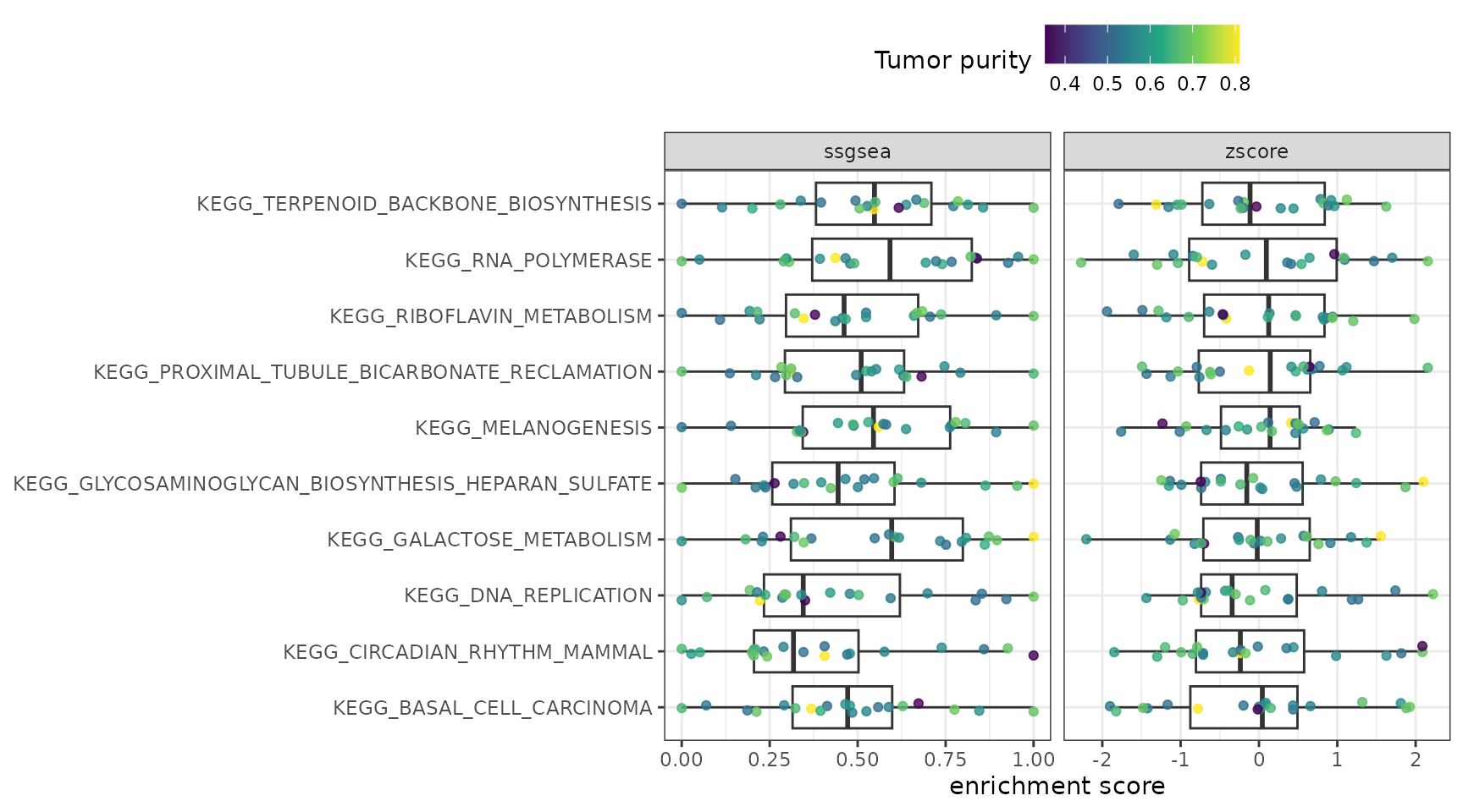
Let’s say we want to compute single sample scores for the KEGG gene set collection and then correlate these scores with the tumor purity given by the ESTIMATE method.

First, we get the KEGG list and use check_sig() to keep only those gene sets whose genes are more than 2/3 present in our gene expression matrix.

kegg_list <- msigdbr(species = "Homo sapiens", subcategory = "KEGG") %>%
    distinct(gs_name, gene_symbol) %>%
    nest(genes = c(gene_symbol)) %>%
    mutate(genes = map(genes, compose(as_vector, unname))) %>%
    deframe()

kegg_ok <- check_sig(test_expr, kegg_list) %>% 
    filter(frac_present > 0.66) %>% 
    pull(signature_id)

Then, we apply both the combined z-score and the ssGSEA method for the resulting list of 10 KEGG gene sets using purrr::map_dfr():

kegg_scores <- map_dfr(list(zscore = "zscore", ssgsea = "ssgsea"), 
                       ~ hack_sig(test_expr,
                                  kegg_list[kegg_ok],
                                  method = .x,
                                  sample_norm = "separate"),
                       .id = "method")

We can transform the kegg_scores tibble in long format using tidyr::pivot_longer():

kegg_scores <- kegg_scores %>% 
    pivot_longer(starts_with("KEGG"), 
                 names_to = "kegg_id", values_to = "kegg_score")

Finally, after computing the tumor purity scores, we can merge the two data sets and plot the results:

purity_scores <- hack_estimate(test_expr) %>% select(sample_id, purity_score)

kegg_scores %>% 
    left_join(purity_scores, by = "sample_id") %>% 
    ggplot(aes(x = kegg_id, y = kegg_score)) +
    geom_boxplot(outlier.alpha = 0) +
    geom_jitter(aes(color = purity_score), alpha = 0.8, width = 0.1) +
    facet_wrap(facets = vars(method), scales = "free_x") +
    coord_flip() +
    scale_color_viridis_c() +
    labs(x = NULL, y = "enrichment score", color = "Tumor purity") +
    theme(legend.position = "top")