10  Distributions

10.1 Bar Plots

10.1.1 A simple bar plot

R

df |> 
    ggplot(aes(gen_health)) +
    geom_bar(color = "red")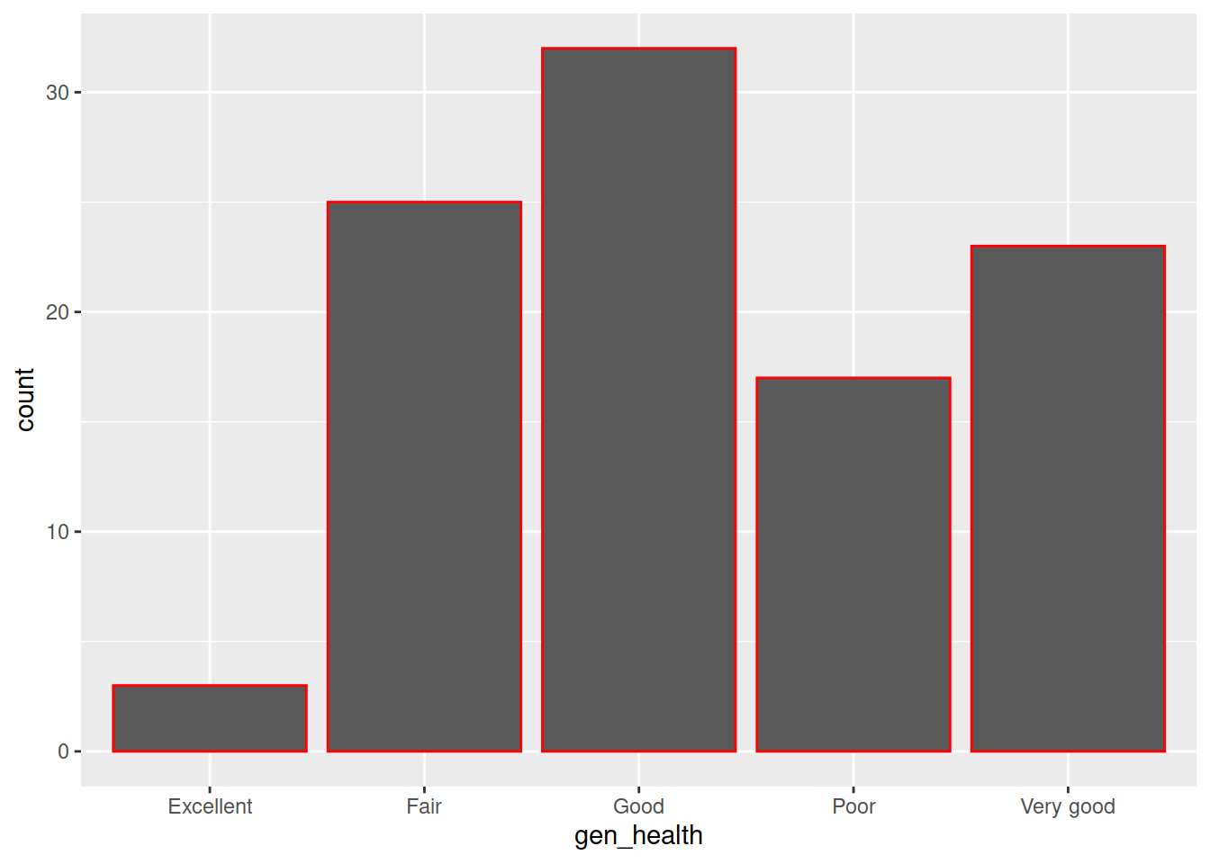

Python

sns.countplot(x="gen_health", color="grey", edgecolor="red", data=df)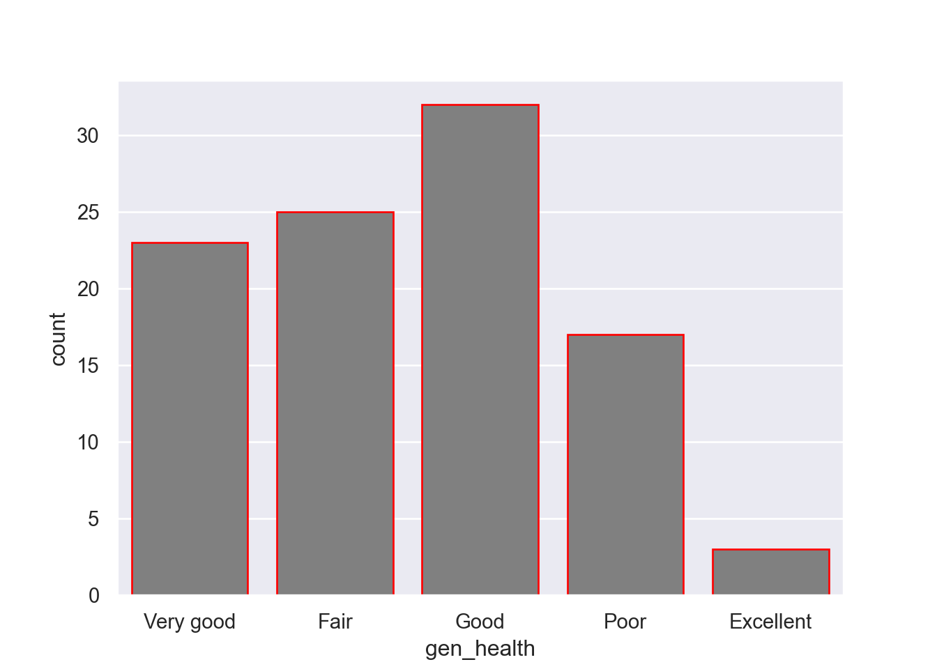

10.1.2 A stacked bar plot

R

df |> 
    ggplot(aes(gen_health, fill = heart_disease)) +
    geom_bar()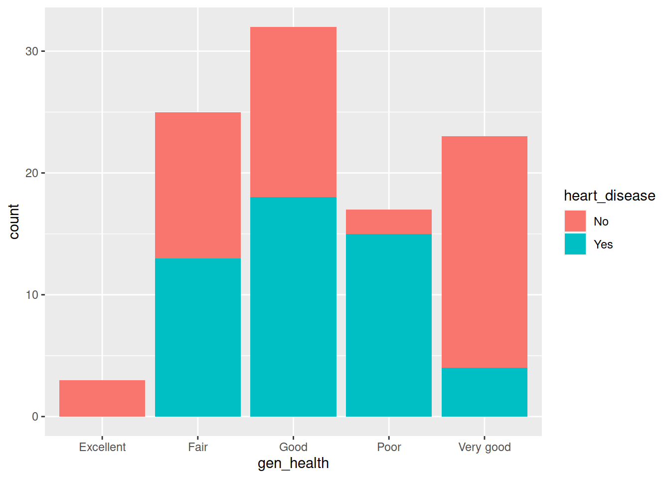

Python

sns.displot(x="gen_health", hue="heart_disease", multiple="stack", aspect=7/5, data=df);
plt.show()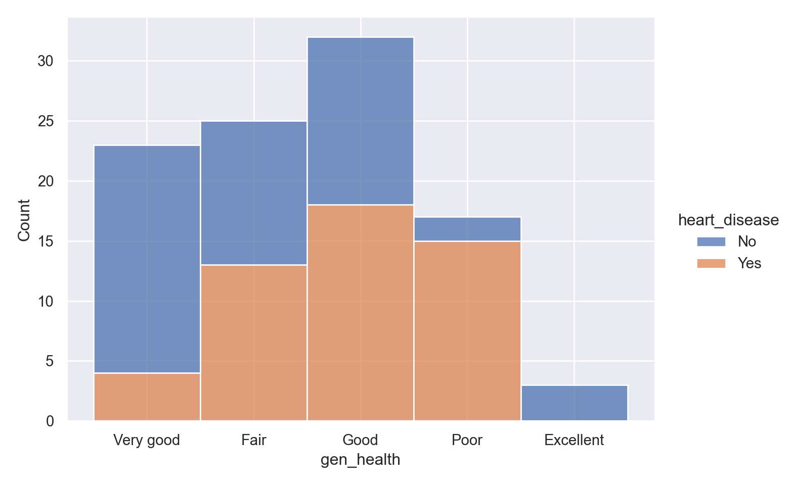

10.1.3 A dodged bar plot

R

df |> 
    ggplot(aes(gen_health, fill = heart_disease)) +
    geom_bar(position = "dodge")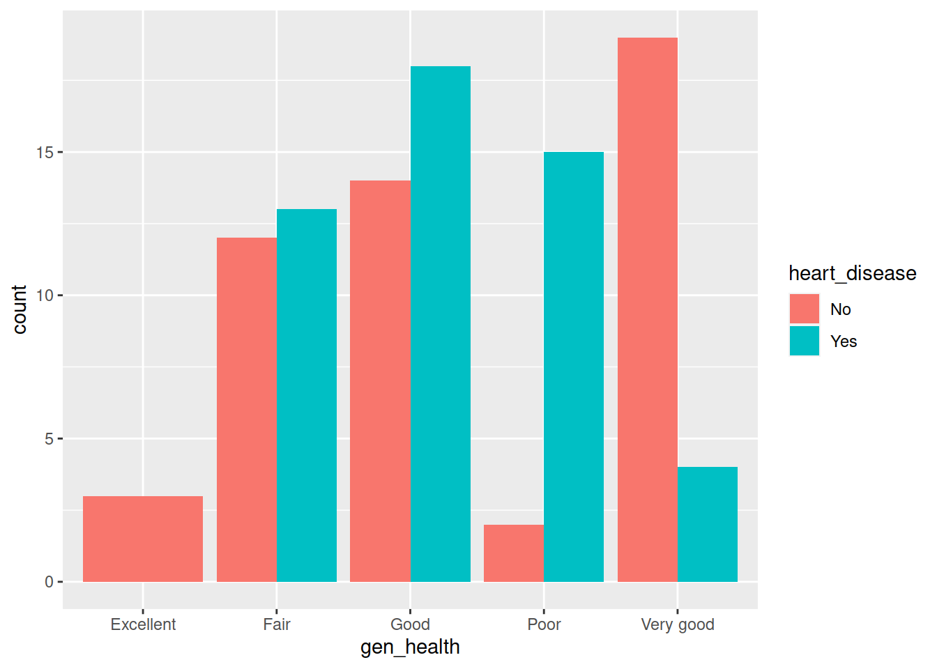

Python

sns.countplot(x="gen_health", hue="heart_disease", data=df)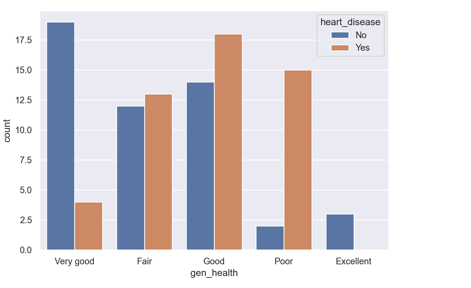

10.2 Histograms

R

df |> 
    ggplot(aes(bmi)) +
    geom_histogram()

`stat_bin()` using `bins = 30`. Pick better value with `binwidth`.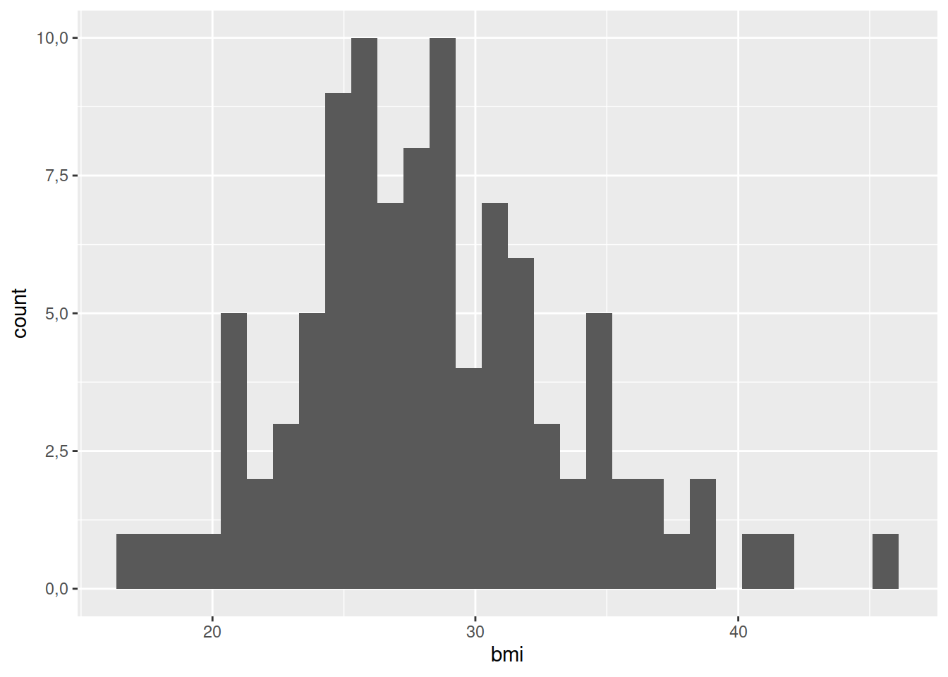

Python

sns.histplot(x="bmi", data=df)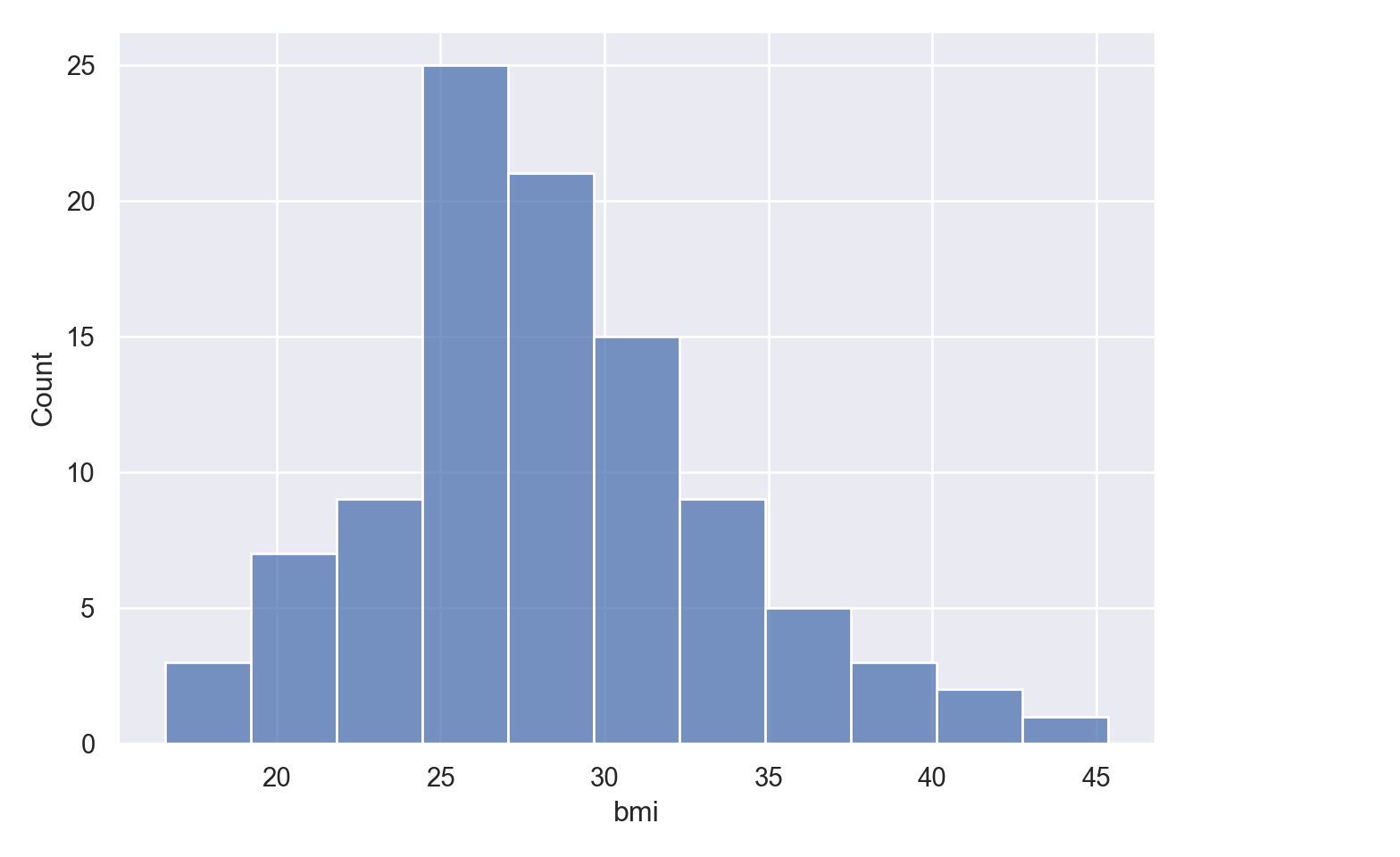

10.3 Density Plots

R

df |> 
    ggplot(aes(bmi)) +
    geom_density()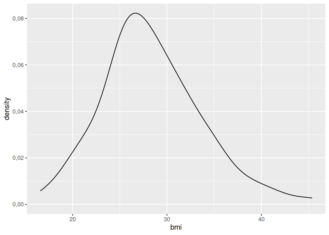

Python

sns.kdeplot(x="bmi", data=df)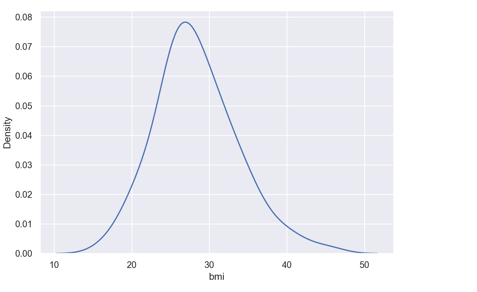

10.4 Boxplots

R

df |> 
    ggplot(aes(smoking, bmi)) +
    geom_boxplot()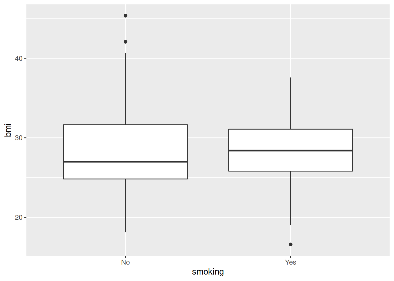

Python

sns.boxplot(x="smoking", y="bmi", data=df)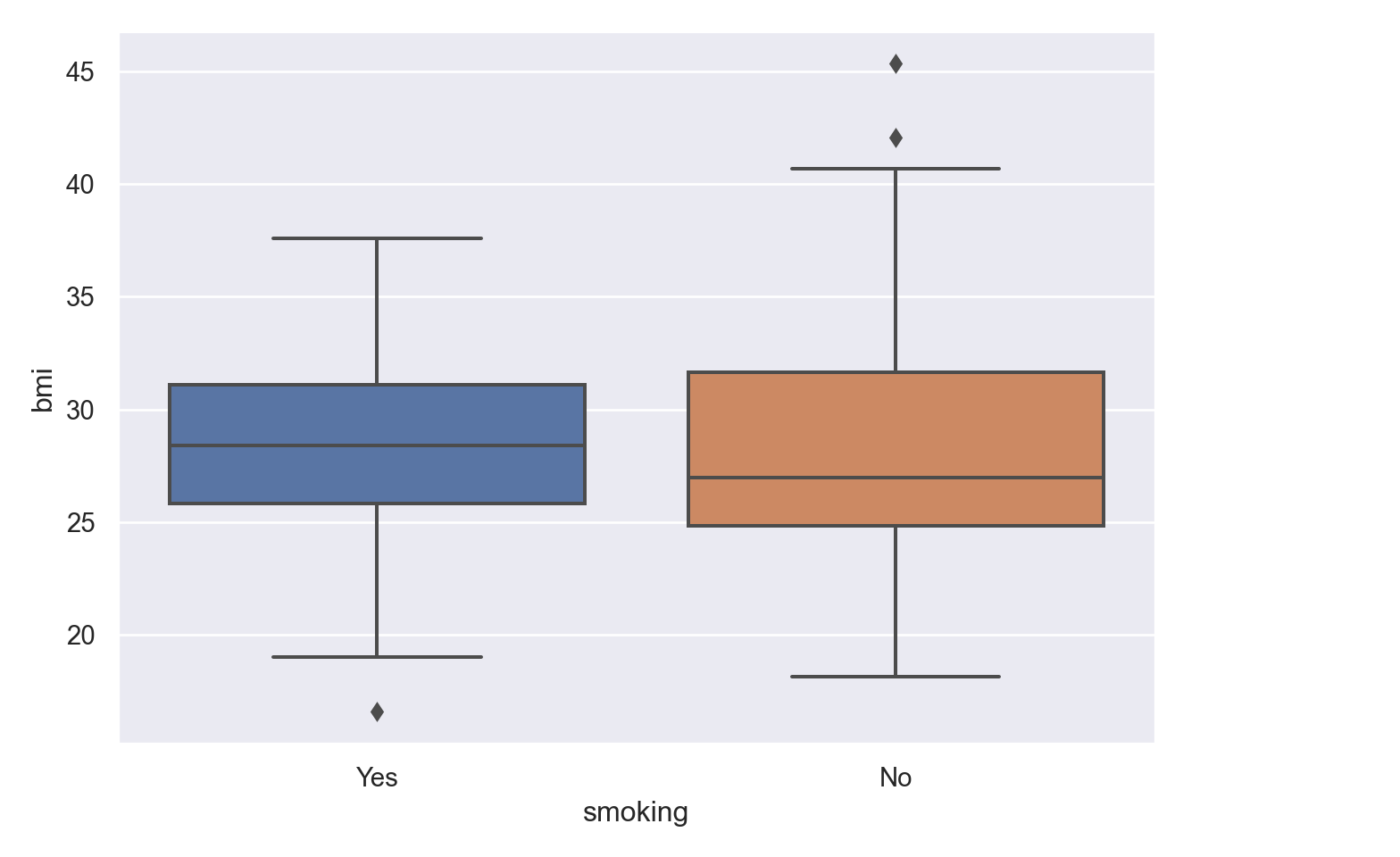

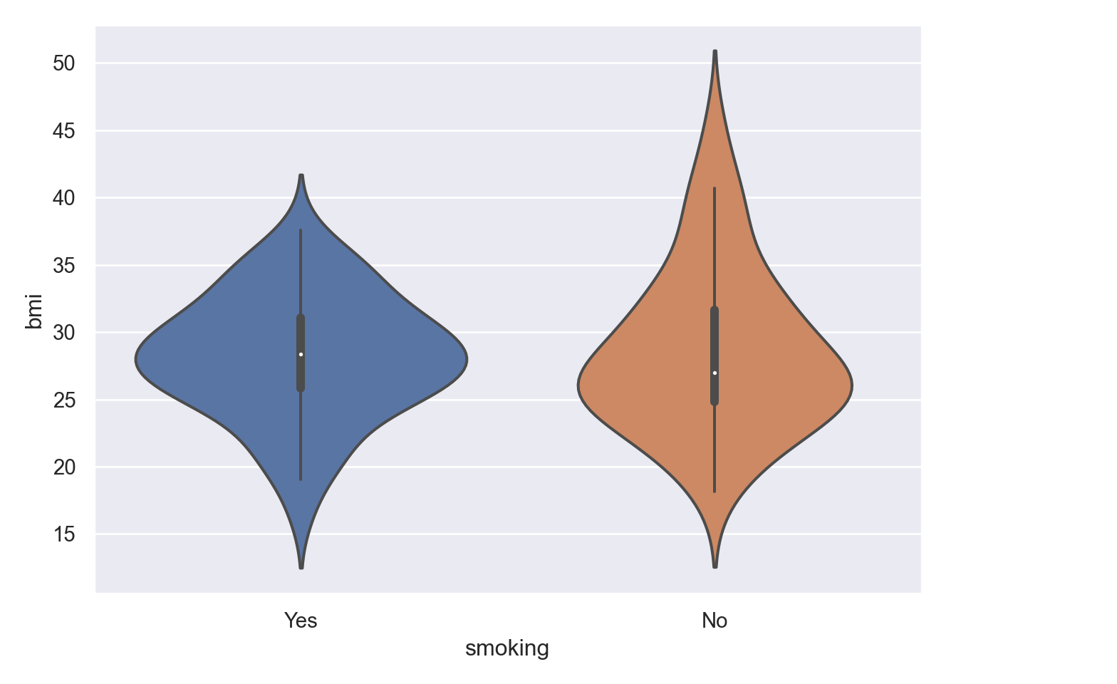
10.5 Violin Plots

R

df |> 
    ggplot(aes(smoking, bmi)) +
    geom_violin()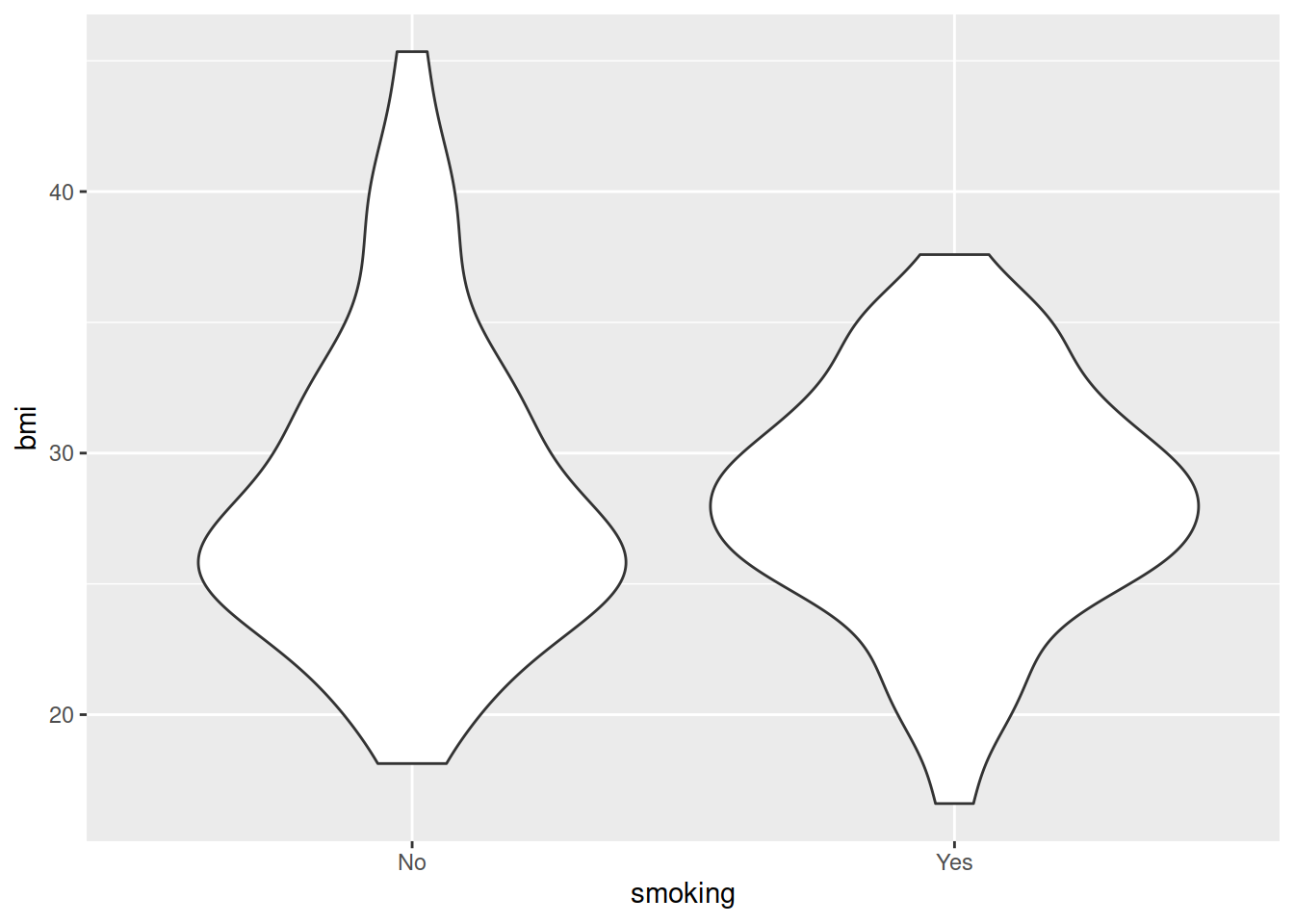

Python

sns.violinplot(x="smoking", y="bmi", data=df)